40 how to add two data labels in excel pie chart
Possible to add second data label to pie chart? - Excel Help Forum Re: Possible to add second data label to pie chart? Create the composite label in a worksheet column by concatenating the data in other cells and the nextline character, CHR (10). Now, use this composite label column as the source for Rob Bovey's add-in. -- Regards, Tushar Mehta Excel, PowerPoint, and VBA add-ins, tutorials Creating Pie Chart and Adding/Formatting Data Labels (Excel) Creating Pie Chart and Adding/Formatting Data Labels (Excel) Creating Pie Chart and Adding/Formatting Data Labels (Excel)
How to Customize Your Excel Pivot Chart Data Labels - dummies The Data Labels command on the Design tab's Add Chart Element menu in Excel allows you to label data markers with values from your pivot table. When you click the command button, Excel displays a menu with commands corresponding to locations for the data labels: None, Center, Left, Right, Above, and Below. None signifies that no data labels should be added to the chart and Show signifies ...
How to add two data labels in excel pie chart
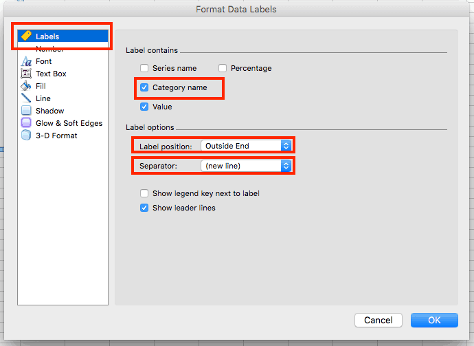
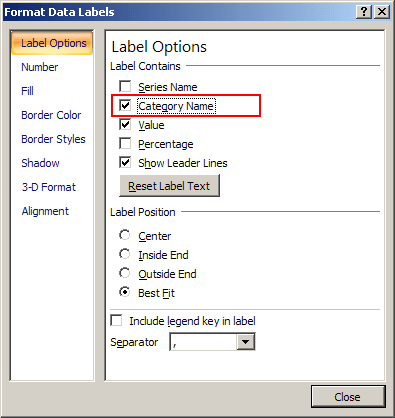
How do I add category labels to a pie chart in Excel? Add data labels Click the chart, and then click the Chart Design tab. Click Add Chart Element and select Data Labels, and then select a location for the data label option. Note: The options will differ depending on your chart type. If you want to show your data label inside a text bubble shape, click Data Callout. How to plot a pie chart in Excel | Basic Excel Tutorial NOTE. 1. On your computer, open the worksheet you want to create a pie chart. 2. In your spreadsheet, select the range of data you want to use for your pie chart. 3. On the main menu ribbon, click on the Insert tab. 4. Here you will see different types of charts, click on the Pie chart icon drop-down arrow. How to Combine or Group Pie Charts in Microsoft Excel Click on the first chart and then hold the Ctrl key as you click on each of the other charts to select them all. Click Format > Group > Group. All pie charts are now combined as one figure. They will move and resize as one image. Choose Different Charts to View your Data
How to add two data labels in excel pie chart. Adding Data Labels to Your Chart (Microsoft Excel) To add data labels in Excel 2013 or Excel 2016, follow these steps: Activate the chart by clicking on it, if necessary. Make sure the Design tab of the ribbon is displayed. (This will appear when the chart is selected.) Click the Add Chart Element drop-down list. Select the Data Labels tool. How to Use Cell Values for Excel Chart Labels - How-To Geek Select the chart, choose the "Chart Elements" option, click the "Data Labels" arrow, and then "More Options.". Uncheck the "Value" box and check the "Value From Cells" box. Select cells C2:C6 to use for the data label range and then click the "OK" button. The values from these cells are now used for the chart data labels. Pie Chart in Excel | How to Create Pie Chart - EDUCBA Step 1: Do not select the data; rather, place a cursor outside the data and insert one PIE CHART. Go to the Insert tab and click on a PIE. Step 2: once you click on a 2-D Pie chart, it will insert the blank chart as shown in the below image. Step 3: Right-click on the chart and choose Select Data. Create two data labels in pie chart? - MrExcel Message Board You have already figured out how to add an image that fills the sector of the pie chart but as far as I know you cannot add an icon or image over the actual pie chart sector, in such a way that it adjusts with the values. If you add it as a static image next to the legend, at least the legend does not move when the values change. Cheers Paul.
How to Create Multi-Category Charts in Excel? - GeeksforGeeks Step 1: Insert the data into the cells in Excel. Now select all the data by dragging and then go to "Insert" and select "Insert Column or Bar Chart". A pop-down menu having 2-D and 3-D bars will occur and select "vertical bar" from it. Select the cell -> Insert -> Chart Groups -> 2-D Column Bar Chart Insertion Multi-Category Chart How To Show Two Sets of Data on One Graph in Excel Below are steps you can use to help add two sets of data to a graph in Excel: 1. Enter data in the Excel spreadsheet you want on the graph. To create a graph with data on it in Excel, the data has to be represented in the spreadsheet. For multiple variables that you want to see plotted on the same graph, entering the values into different ... Create a multi-level category chart in Excel - ExtendOffice Double click any series in the chart to open the Format Data Series pane. In the pane, change the Gap Width to 0%. 5. Select the spacing1 data series in the chart, go to the Format Data Series pane to configure as follows. 5.1) Click the Fill & Line icon; 5.2) Select No fill in the Fill section. Then these data bars are hidden. 6. How to group (two-level) axis labels in a chart in Excel? (1) In Excel 2007 and 2010, clicking the PivotTable > PivotChart in the Tables group on the Insert Tab; (2) In Excel 2013, clicking the Pivot Chart > Pivot Chart in the Charts group on the Insert tab. 2. In the opening dialog box, check the Existing worksheet option, and then select a cell in current worksheet, and click the OK button. 3.
How to Add Data Labels to an Excel 2010 Chart - dummies Use the following steps to add data labels to series in a chart: Click anywhere on the chart that you want to modify. On the Chart Tools Layout tab, click the Data Labels button in the Labels group. A menu of data label placement options appears: None: The default choice; it means you don't want to display data labels. How to add data labels from different column in an Excel chart? Right click the data series in the chart, and select Add Data Labels > Add Data Labels from the context menu to add data labels. 2. Click any data label to select all data labels, and then click the specified data label to select it only in the chart. 3. Change the format of data labels in a chart To get there, after adding your data labels, select the data label to format, and then click Chart Elements > Data Labels > More Options. To go to the appropriate area, click one of the four icons ( Fill & Line, Effects, Size & Properties ( Layout & Properties in Outlook or Word), or Label Options) shown here. How to show percentage in pie chart in Excel? - ExtendOffice Please do as follows to create a pie chart and show percentage in the pie slices. 1. Select the data you will create a pie chart based on, click Insert > I nsert Pie or Doughnut Chart > Pie. See screenshot: 2. Then a pie chart is created. Right click the pie chart and select Add Data Labels from the context menu. 3.
How to Create a Pie Chart in Excel | Smartsheet
Add data labels and callouts to charts in Excel 365 - EasyTweaks.com Step #1: After generating the chart in Excel, right-click anywhere within the chart and select Add labels . Note that you can also select the very handy option of Adding data Callouts. Step #2: When you select the "Add Labels" option, all the different portions of the chart will automatically take on the corresponding values in the table ...

Excel 3-D Pie Charts
how to make a pie chart in canva - The Blue Monkey Restaurant & Pizzeria Creating Your Pie Chart. First, go up to the "Insert" tab at the top of your screen. Add shape in Google slides. Then, go down to the "Shape" option. Under "Shape," go over to the "Shapes" sub-option, and select the shape of the pie chart. Finally, you'll click and drag to create the pie.
Excel 3-D Pie charts - Microsoft Excel 2007
How To Create A Pie Chart In Excel (With Percentages) - YouTube In this video, I'm going to show you how to create a pie chart by using Microsoft Excel. I will show you how to add data labels that are percentages and even...
How to Make a Pie Chart in Excel & Add Rich Data Labels to The Chart!
Pie of Pie Chart in Excel - Inserting, Customizing, Formatting To add the data labels:- Select the chart and click on + icon at the top right corner of chart. Mark the check box containing data labels. Formatting Data Labels Consequently, this is going to insert default data labels on the chart.
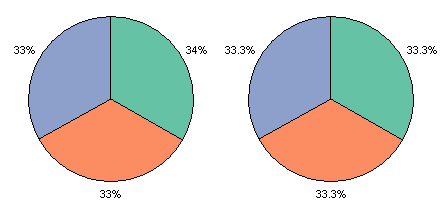
Pie Chart Rounding in Excel - Peltier Tech
Excel charts: add title, customize chart axis, legend and data labels ... Click anywhere within your Excel chart, then click the Chart Elements button and check the Axis Titles box. If you want to display the title only for one axis, either horizontal or vertical, click the arrow next to Axis Titles and clear one of the boxes: Click the axis title box on the chart, and type the text.
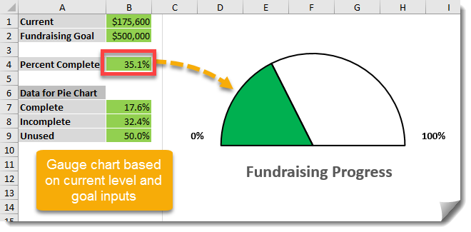
How To Create A Gauge Chart For Measuring Progress Against A Goal | How To Excel
How to Create and Format a Pie Chart in Excel - Lifewire To add data labels to a pie chart: Select the plot area of the pie chart. Right-click the chart. Select Add Data Labels . Select Add Data Labels. In this example, the sales for each cookie is added to the slices of the pie chart. Change Colors
EXCEL Charts: Column, Bar, Pie and Line
Edit titles or data labels in a chart - support.microsoft.com On a chart, click one time or two times on the data label that you want to link to a corresponding worksheet cell. The first click selects the data labels for the whole data series, and the second click selects the individual data label. Right-click the data label, and then click Format Data Label or Format Data Labels.
Post a Comment for "40 how to add two data labels in excel pie chart"