45 how to display data labels in excel
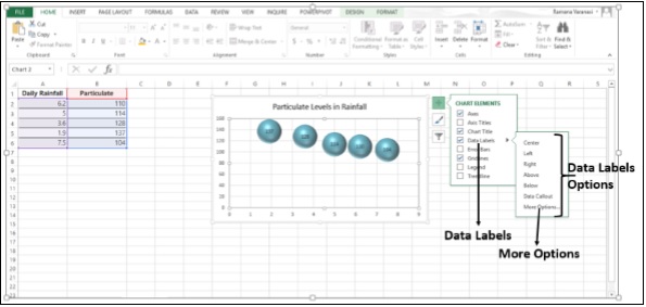
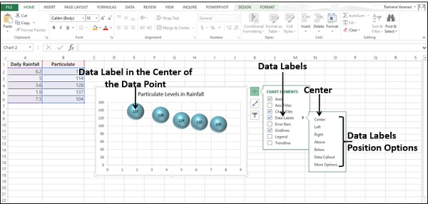
How to add or move data labels in Excel chart? - ExtendOffice 1. Click the chart to show the Chart Elements button . 2. Then click the Chart Elements, and check Data Labels, then you can click the arrow to choose an option about the data labels in the sub menu. See screenshot: How to Insert Axis Labels In An Excel Chart | Excelchat We will again click on the chart to turn on the Chart Design tab. We will go to Chart Design and select Add Chart Element. Figure 6 - Insert axis labels in Excel. In the drop-down menu, we will click on Axis Titles, and subsequently, select Primary vertical. Figure 7 - Edit vertical axis labels in Excel. Now, we can enter the name we want ...
Custom Chart Data Labels In Excel With Formulas Follow the steps below to create the custom data labels. Select the chart label you want to change. In the formula-bar hit = (equals), select the cell reference containing your chart label's data. In this case, the first label is in cell E2. Finally, repeat for all your chart laebls.

How to display data labels in excel
Excel Charts: Dynamic Label positioning of line series - XelPlus Go to Layout tab, select Data Labels > Right. Right mouse click on the data label displayed on the chart. Select Format Data Labels. Under the Label Options, show the Series Name and untick the Value. Show the Label Instead of the Value for Actual How to Use Cell Values for Excel Chart Labels Select the chart, choose the "Chart Elements" option, click the "Data Labels" arrow, and then "More Options." Uncheck the "Value" box and check the "Value From Cells" box. Select cells C2:C6 to use for the data label range and then click the "OK" button. The values from these cells are now used for the chart data labels. Format Data Labels in Excel- Instructions - TeachUcomp, Inc. To do this, click the "Format" tab within the "Chart Tools" contextual tab in the Ribbon. Then select the data labels to format from the "Chart Elements" drop-down in the "Current Selection" button group. Then click the "Format Selection" button that appears below the drop-down menu in the same area.
How to display data labels in excel. How to Customize Your Excel Pivot Chart Data Labels - dummies When you click the command button, Excel displays a menu with commands corresponding to locations for the data labels: None, Center, Left, Right, Above, and Below. None signifies that no data labels should be added to the chart and Show signifies heck yes, add data labels. The menu also displays a More Data Label Options command. Add or remove data labels in a chart - support.microsoft.com Right-click the data series or data label to display more data for, and then click Format Data Labels. Click Label Options and under Label Contains, select the Values From Cells checkbox. When the Data Label Range dialog box appears, go back to the spreadsheet and select the range for which you want the cell values to display as data labels. Office: Display Data Labels in a Pie Chart - Tech-Recipes 3. In the Chart window, choose the Pie chart option from the list on the left. Next, choose the type of pie chart you want on the right side. 4. Once the chart is inserted into the document, you will notice that there are no data labels. To fix this problem, select the chart, click the plus button near the chart's bounding box on the right ... Change the format of data labels in a chart To get there, after adding your data labels, select the data label to format, and then click Chart Elements > Data Labels > More Options. To go to the appropriate area, click one of the four icons ( Fill & Line, Effects, Size & Properties ( Layout & Properties in Outlook or Word), or Label Options) shown here.
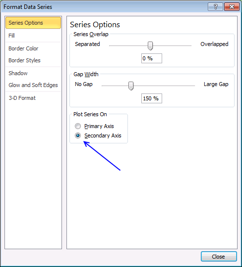
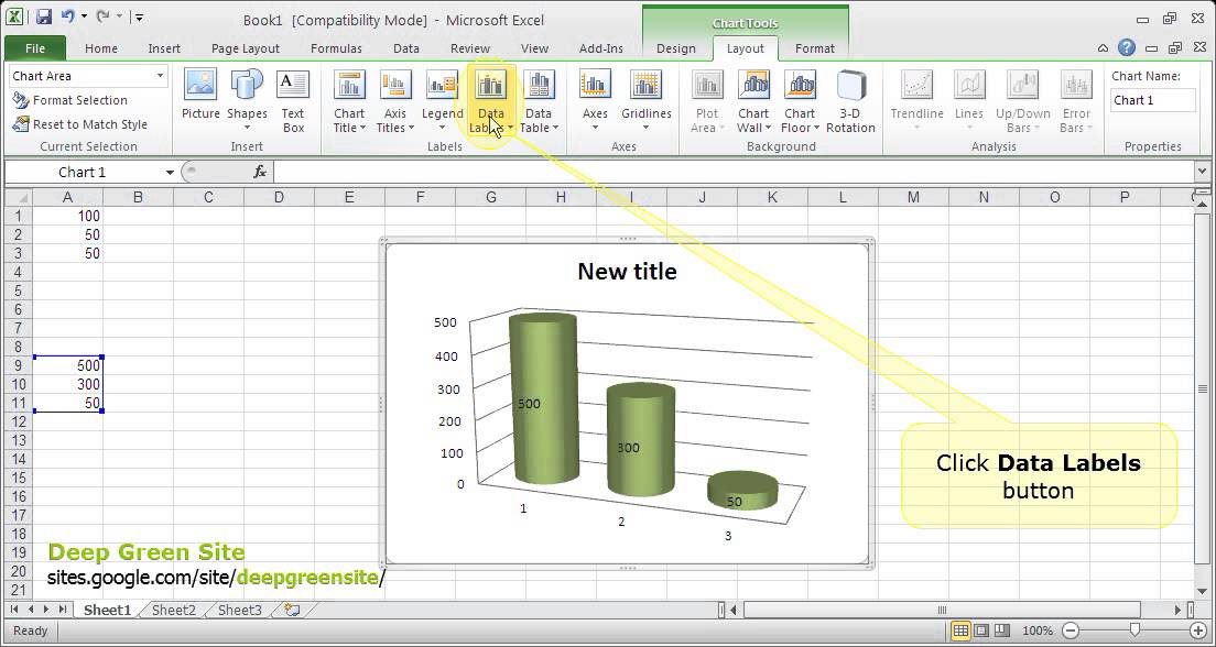
Excel tutorial: How to use data labels Generally, the easiest way to show data labels to use the chart elements menu. When you check the box, you'll see data labels appear in the chart. If you have more than one data series, you can select a series first, then turn on data labels for that series only. You can even select a single bar, and show just one data label. How to Add Labels to Show Totals in Stacked Column Charts in Excel In the chart, right-click the "Total" series and then, on the shortcut menu, select Add Data Labels. 9. Next, select the labels and then, in the Format Data Labels pane, under Label Options, set the Label Position to Above. 10. While the labels are still selected set their font to Bold. 11. Chart: Display alternative values as Data Labels or Data Callouts - MrExcel Joined. Aug 11, 2017. Messages. 1. Aug 11, 2017. #1. Below is my excel chart. I would like to add a "data labels" or "data callouts". As you can see the line is displaying the data from Actual X and Y, but I want to display the DEV values on this line. How to Add Data Labels to an Excel 2010 Chart - dummies On the Chart Tools Layout tab, click Data Labels→More Data Label Options. The Format Data Labels dialog box appears. You can use the options on the Label Options, Number, Fill, Border Color, Border Styles, Shadow, Glow and Soft Edges, 3-D Format, and Alignment tabs to customize the appearance and position of the data labels.
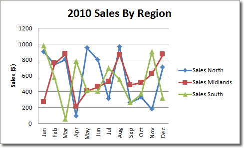
Excel charts: add title, customize chart axis, legend and data labels ... Click anywhere within your Excel chart, then click the Chart Elements button and check the Axis Titles box. If you want to display the title only for one axis, either horizontal or vertical, click the arrow next to Axis Titles and clear one of the boxes: Click the axis title box on the chart, and type the text. Understanding Excel Chart Data Series, Data Points, and Data Labels Numeric Values: Taken from individual data points in the worksheet. Series Names: Identifies the columns or rows of chart data in the worksheet. Series names are commonly used for column charts, bar charts, and line graphs. Category Names: Identifies the individual data points in a single series of data. These are commonly used for pie charts. How to find, highlight and label a data point in Excel scatter plot Select the Data Labels box and choose where to position the label. By default, Excel shows one numeric value for the label, y value in our case. To display both x and y values, right-click the label, click Format Data Labels…, select the X Value and Y value boxes, and set the Separator of your choosing: Label the data point by name How to use data labels in a chart - YouTube Excel charts have a flexible system to display values called "data labels". Data labels are a classic example a "simple" Excel feature with a huge range of o...

Pie Chart - PK: An Excel Expert
Dynamic Chart Data Labels : excel Currently, my background is white, bar chart is red, data labels are white. For the most part this works fine. However, when a particular filter on the slicer is selected, one of the bar has a very small value and the data label exceeds the bar. Since the data label font is white and the background is white, im not able to see the data label.
How to add live total labels to graphs and charts in Excel and PowerPoint | BrightCarbon
Quick Tip: Excel 2013 offers flexible data labels | TechRepublic right-click and choose Insert Data Label Field. In the next dialog, select [Cell] Choose Cell. When Excel displays the source dialog, click the cell that contains the MIN () function, and click OK....
Custom data labels in a chart | Get Digital Help - Microsoft Excel resource
How to add data labels from different column in an Excel chart? Click any data label to select all data labels, and then click the specified data label to select it only in the chart. 3. Go to the formula bar, type =, select the corresponding cell in the different column, and press the Enter key. See screenshot: 4. Repeat the above 2 - 3 steps to add data labels from the different column for other data points.
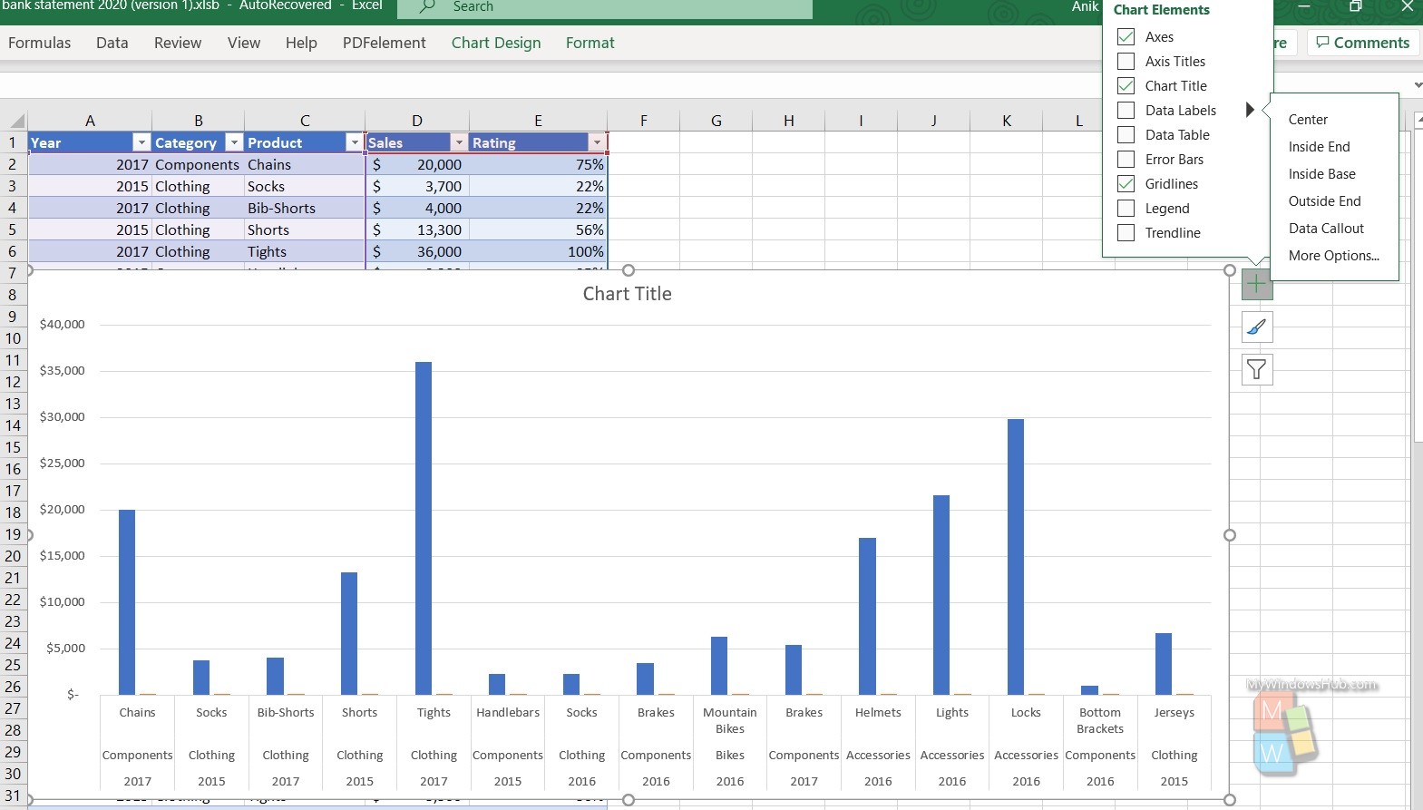
How To Show Or Hide Data Labels On MS Excel? | My Windows Hub
How to Add Labels to Scatterplot Points in Excel - Statology Step 3: Add Labels to Points Next, click anywhere on the chart until a green plus (+) sign appears in the top right corner. Then click Data Labels, then click More Options… In the Format Data Labels window that appears on the right of the screen, uncheck the box next to Y Value and check the box next to Value From Cells.

Format Data Labels in Excel- Instructions | Microsoft excel, Microsoft, Bar chart
How to Change Excel Chart Data Labels to Custom Values? Now, click on any data label. This will select "all" data labels. Now click once again. At this point excel will select only one data label. Go to Formula bar, press = and point to the cell where the data label for that chart data point is defined. Repeat the process for all other data labels, one after another. See the screencast. Points to note:
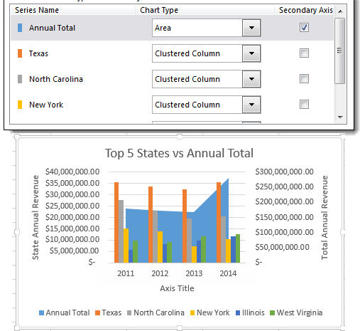
Working with Multiple Data Series in Excel | Pryor Learning Solutions
Excel charts: how to move data labels to legend - Microsoft Tech Community You can't do that, but you can show a data table below the chart instead of data labels: Click anywhere on the chart. On the Design tab of the ribbon (under Chart Tools), in the Chart Layouts group, click Add Chart Element > Data Table > With Legend Keys (or No Legend Keys if you prefer)

How to Create Progress Charts (Bar and Circle) in Excel - Automate Excel
How to show data label in "percentage" instead of - Microsoft Community Select Format Data Labels Select Number in the left column Select Percentage in the popup options In the Format code field set the number of decimal places required and click Add. (Or if the table data in in percentage format then you can select Link to source.) Click OK Regards, OssieMac Report abuse 8 people found this reply helpful ·
November 2018
Enable or Disable Excel Data Labels at the click of a button - How To Step 1: Here is the sample data. Select and to go Insert tab > Charts group > Click column charts button > click 2D column chart. This will insert a new chart in the worksheet. Step 2: Having chart selected go to design tab > click add chart element button > hover over data labels > click outside end or whatever you feel fit.

Format Number Options for Chart Data Labels in Excel 2011 for Mac
How to Display a Label Within a Formula on Excel - YouTube Subscribe Now: More: a label within a formula on Ex...

GANTT Procedure
Format Data Labels in Excel- Instructions - TeachUcomp, Inc. To do this, click the "Format" tab within the "Chart Tools" contextual tab in the Ribbon. Then select the data labels to format from the "Chart Elements" drop-down in the "Current Selection" button group. Then click the "Format Selection" button that appears below the drop-down menu in the same area.

Label Printing Software - Print Barcode Labels from Excel, Access, C#, VB.NET
How to Use Cell Values for Excel Chart Labels Select the chart, choose the "Chart Elements" option, click the "Data Labels" arrow, and then "More Options." Uncheck the "Value" box and check the "Value From Cells" box. Select cells C2:C6 to use for the data label range and then click the "OK" button. The values from these cells are now used for the chart data labels.
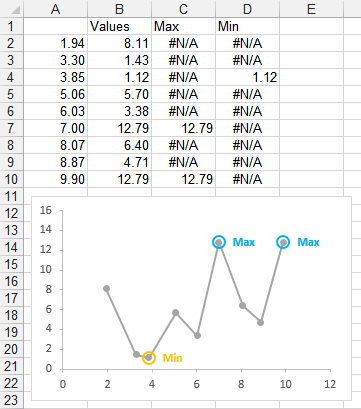
Highlight Minimum and Maximum in an Excel Chart - Peltier Tech
Excel Charts: Dynamic Label positioning of line series - XelPlus Go to Layout tab, select Data Labels > Right. Right mouse click on the data label displayed on the chart. Select Format Data Labels. Under the Label Options, show the Series Name and untick the Value. Show the Label Instead of the Value for Actual
Advanced Excel - более богатые метки данных - CoderLessons.com
Excel Dashboards - Краткое руководство - CoderLessons.com
Excel - Line Chart

How to Make an Excel Histogram Display the Data Distribution - My Microsoft Office Tips
MS Excel 2010 / How to remove data labels from the chart - YouTube

31 What Is Data Label In Excel - Labels Database 2020
Post a Comment for "45 how to display data labels in excel"